The Coefficients' Shrinkage Path of Ridge and Lasso Regression
- Karl 曹
- Sep 25, 2022
- 4 min read
Here we compare the shrinkage path of Ridge and Lasso regression, here the shrinkage path refers to the different coefficients of different tuning parameters. Because after we know how parameters perform, we can better understand how shrinkage methods work.
We use the following data generating process as baseline setting:

the true beta vector is (0.5 0.5 -0.5)
variance-covariance matrix sigma is
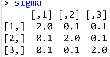
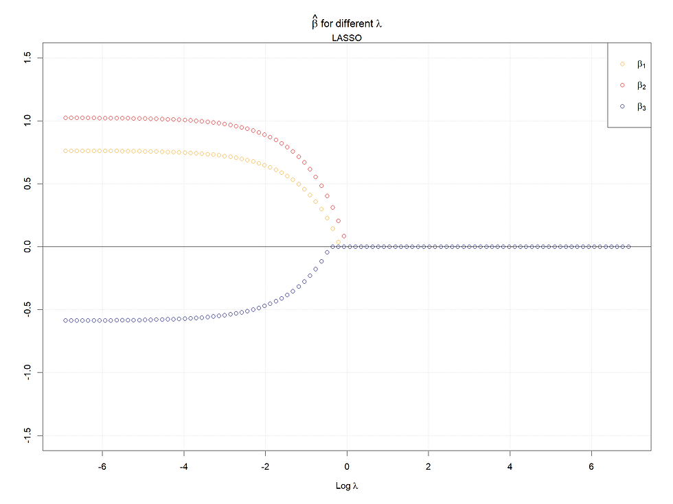
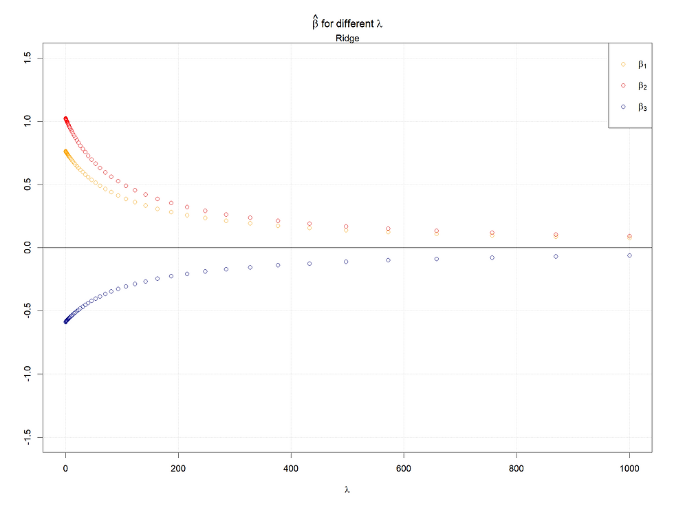
Case 1, the baseline case:
Note that the horizontal axis of the Lasso figure is the logged tuning parameter interval.
Case 2: Variables with different variance
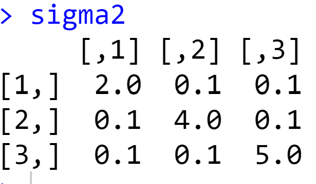
Here we change the var-covariance matrix, let X2 and X3 have larger variances, and covariance keeps the same as before. However, for both shrinkage methods, standardization is recommended, and here both regressions are done with standardized data, thus case 2 makes less sense, and the explanation of cases 1 and 2 should be the same :)

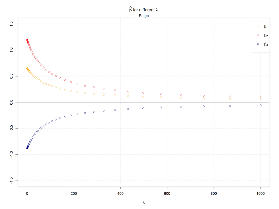
Both in cases 1 & 2, for Lasso, the larger (absolute value) the coefficients when lambda is 0, the later the coefficients shrink to 0 as lambda increases. Meanwhile, for the ridge regression, rather than shrinking to 0, their values decrease faster given a smaller (absolutely) coefficient (when lambda = 0).
Case 3: High correlated variables
We can set X1 and X2 are highly correlated.
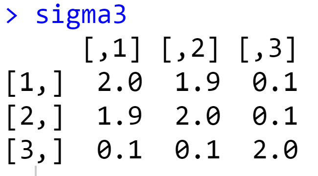
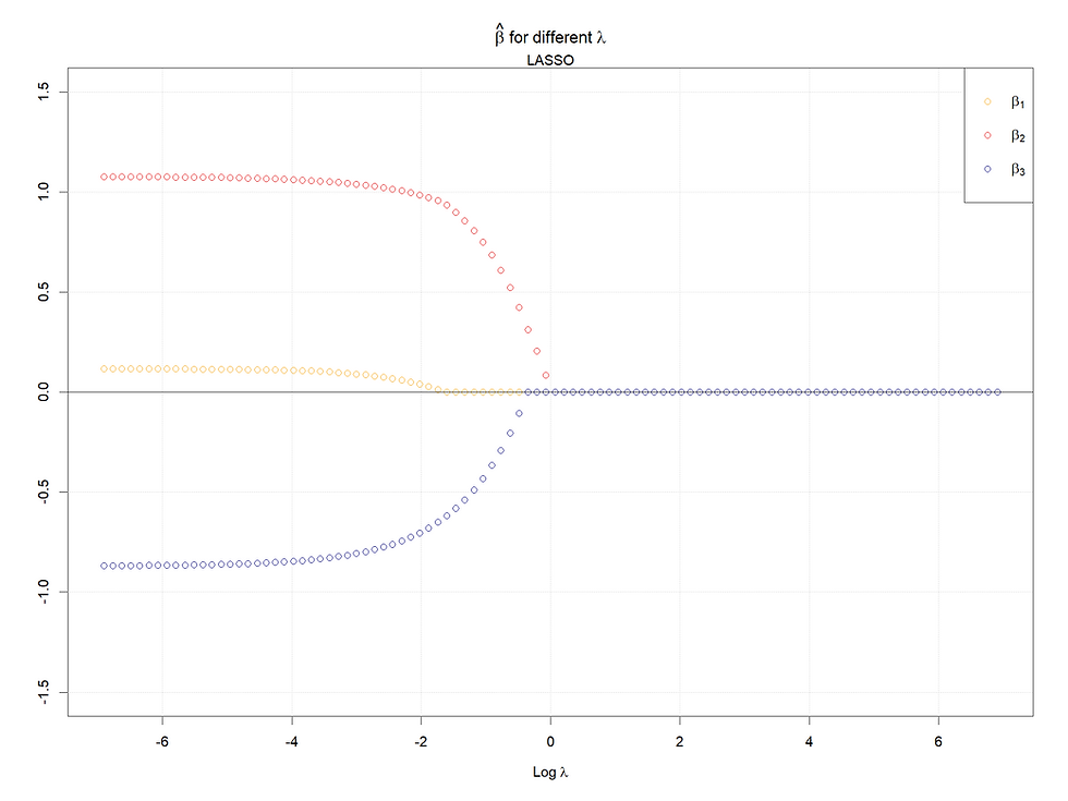
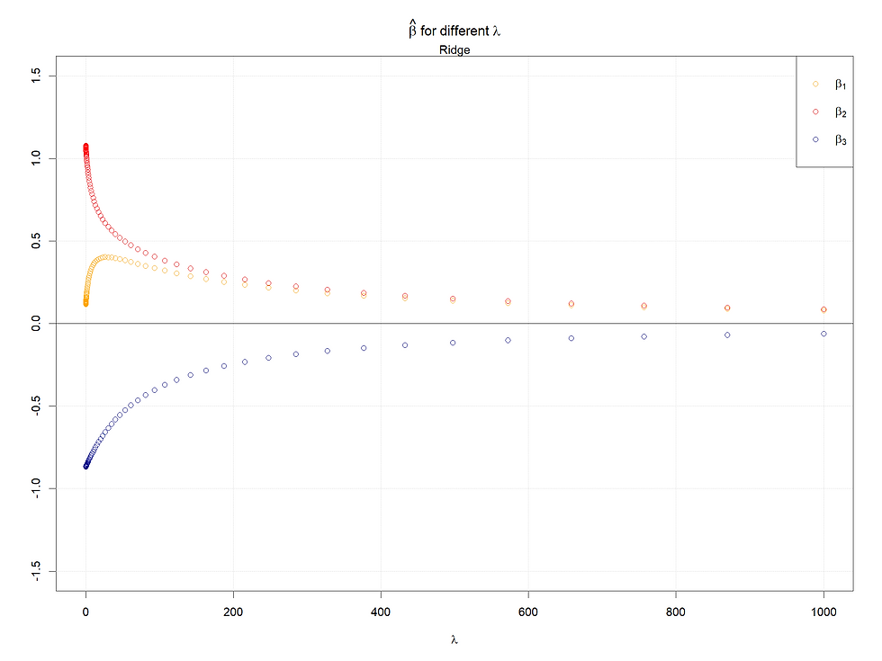
Here we see that X1's lambda 0 coefficient becomes very small and X2's becomes around 1, which makes sense because either X1 or X2 can reflect most information given high covariance.
And here we can observe the difference between Ridge and Lasso. For ridge, the two coefficients' path converges to each other, but for the Lasso case, the coefficient of X1 quickly goes to 0. Here we can see the different logic of shrinkage methods of these two. In summary, Ridge makes two coefficients simultaneously decrease, but Lasso drops one of them.
Case 4: High correlation of X1 and X3


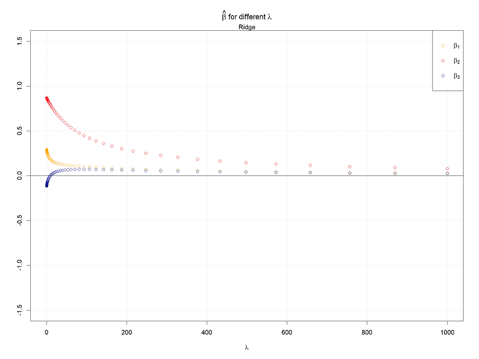
Here we observe the same pattern as in case 3. However, for the Lasso case, we can see that when the coefficient of X3 becomes 0, the path of X1 changes its decrease pattern, because when X3 plays no role, the highly correlated X1 takes more influence, then we see the steep decrease pattern suddenly becomes to a smother pattern.
Case 5: All variables are highly correlated
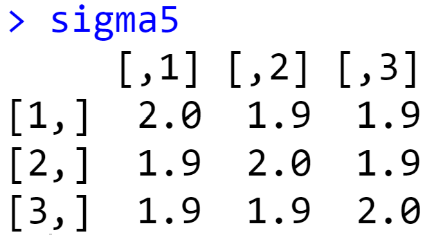

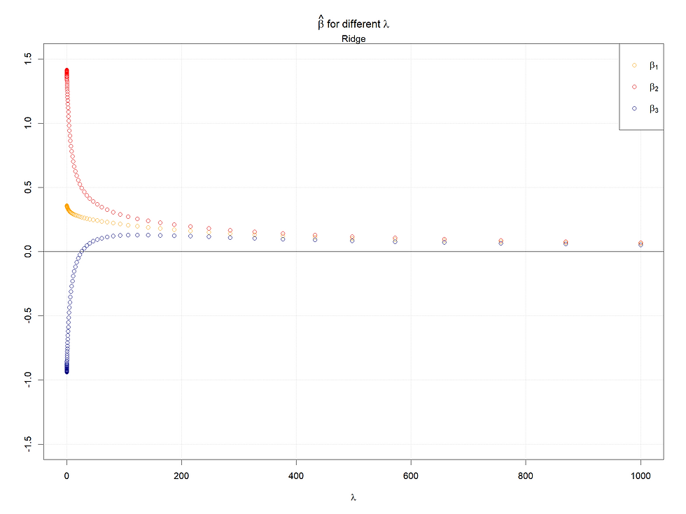
As in case 4, we can see the same pattern, the kink also exists in the Lasso case.
In conclusion, the larger the starting points of coefficients (refers to 0 lambda), the later the coefficients shrink to 0 or small values. Meanwhile, for highly correlated variables, the Ridge will make them converge to the same value as lambda increases, and in the Lasso case, one of the set of highly correlated variables will shrink to 0 firstly and quickly, at the same time a kink will appear at the paths left.
R code:
# test the shrinkage path of ridge and Lasso
rm(list = ls())
library(glmnet)
library(MASS)
set.seed(777)
n <- 100
beta.true <- c(0.5, 0.5, -0.5)
sigma <- matrix(c(2,0.1,0.1,
                  0.1,2,0.1,
                  0.1,0.1,2) ,
                nrow= 3, ncol= 3, byrow=TRUE)

sigma2 <- matrix(c(2,0.1,0.1,
                  0.1,4,0.1,
                  0.1,0.1,5) ,
                nrow= 3, ncol= 3, byrow=TRUE)
sigma3 <- matrix(c(2,1.9,0.1,
                  1.9,2,0.1,
                  0.1,0.1,2) ,
                nrow= 3, ncol= 3, byrow=TRUE)
sigma4 <- matrix(c(2,0.1,1.9,
                  0.1,2,0.1,
                  1.9,0.1,2) ,
                nrow= 3, ncol= 3, byrow=TRUE)
sigma5 <- matrix(c(2,1.9,1.9,
                  1.9,2,1.9,
                  1.9,1.9,2) ,
                nrow= 3, ncol= 3, byrow=TRUE)
mu <- rep(0,3)
data.generator <- function(n, sigma, mu, beta){
  x <- mvrnorm(n, mu, sigma)
  e <- rnorm(n, 0, sqrt(10))
  y <- x %*% beta + e
  x.1 <- x[,1] / sd(x[,1])
  x.2 <- x[,2]/ sd(x[,2])
  x.3 <- x[,3]/ sd(x[,3])
  x.sd <- cbind(x.1, x.2, x.3)
  data <- data.frame ("y" = y, "x.sd" = x.sd, "x" = x)
  return(data)
}

set.seed(777)
data <- data.generator(n, sigma, mu, beta.true)
set.seed(777)
data <- data.generator(n, sigma2, mu, beta.true)
set.seed(777)
data <- data.generator(n, sigma3, mu, beta.true)
set.seed(777)
data <- data.generator(n, sigma4, mu, beta.true)
set.seed(777)
data <- data.generator(n, sigma5, mu, beta.true)

x.sd <- cbind(data$x.sd.x.1, data$x.sd.x.2, data$x.sd.x.3)
x <- cbind(data$x.1, data$x.2, data$x.3)
ridge <- function(x,y,lambda, p = 3){
  beta.ridge <- solve(t(x) %*% x +
                        diag(lambda, nrow = p, ncol = p)) %*% t(x) %*% y
  return(beta.ridge)
}
grid <- 10^ seq (3, -3, length = 100)
beta.ridge <- matrix(NA, nrow = 3, ncol= length(grid))
beta.ridge.nonsd <- matrix(NA, nrow = 3, ncol= length(grid))
for (i in 1:length(grid)){
  lam <- grid[i]
  beta.ridge[,i] <- ridge(x.sd, data$y, lam)
}
for (i in 1:length(grid)){
  lam <- grid[i]
  beta.ridge.nonsd[,i] <- ridge(x, data$y, lam)
}

### Lasso
lasso.mod<-glmnet(x.sd,data$y, alpha=1, lambda = grid,intercept=F)
lassobeta <- as.matrix(lasso.mod$beta)
plot(lasso.mod)

ylimits = c(-1.5, 1.5)
plot(x=log(grid), y=lassobeta[1,], col = "red", ylim = ylimits,
     xlab = expression(Log~lambda), ylab = "",
     main = expression(hat(beta) ~ "for different" ~ lambda), type = "n")
grid()
points(x=log(grid), y=lassobeta[1,], col = "orange", lwd = 1)
points(x=log(grid), y=lassobeta[2,], col = "red", lwd = 1)
points(x=log(grid), y=lassobeta[3,], col = "darkblue", lwd = 1)
abline(h = 0, col = "black")
legend("topright", c(expression(beta[1]), expression(beta[2]), expression(beta[3])),
       col = c("orange", "red", "darkblue"), pch = 1)
mtext("LASSO")


ylimits = c(-1.5, 1.5)
plot(x=grid, y=beta.ridge[1,], col = "red", ylim = ylimits,
     xlab = expression(lambda), ylab = "",
     main = expression(hat(beta) ~ "for different" ~ lambda), type = "n")
grid()
points(x=grid, y=beta.ridge[1,], col = "orange", lwd = 1)
points(x=grid, y=beta.ridge[2,], col = "red", lwd = 1)
points(x=grid, y=beta.ridge[3,], col = "darkblue", lwd = 1)
abline(h = 0, col = "black")
legend("topright", c(expression(beta[1]), expression(beta[2]), expression(beta[3])),
       col = c("orange", "red", "darkblue"), pch = 1)
mtext("Ridge")


Comments